How to plot and understand turbulence using the brightwind library

---

import datetime
print('Last updated: {}'.format(datetime.date.today().strftime('%d %B, %Y')))

Last updated: 03 July, 2019

---

Outline:

This guide will demonstrate how to get some useful turbulence intensity statistics from a sample dataset using the following steps:

• Import the brightwind library and some sample data

• Plot the turbulence intensity by direction

• Clean out some bad data and replot the turbulence intensity

• Plot the turbulence intensity by windspeed and get access to the underlying data

• Calculate a 12x24 matrix of turbulence intensity

---

Load some data

import brightwind as bw

# specify file location of existing sample dataset
filepath = r'C:\Users\Stephen\Documents\Analysis\demo_data.csv'
# load data into a dataframe
data = bw.load_csv(filepath)
# show first few rows of dataframe
data.head(5)

	Spd80mN	Spd80mS	Spd60mN	Spd60mS	Spd40mN	Spd40mS	Spd80mNStd	Spd80mSStd	Spd60mNStd	Spd60mSStd	...	Dir78mSStd	Dir58mS	Dir58mSStd	Dir38mS	Dir38mSStd	T2m	RH2m	P2m	PrcpTot	BattMin
Timestamp
2016-01-09 15:30:00	8.370	7.911	8.160	7.849	7.857	7.626	1.240	1.075	1.060	0.947	...	6.100	110.1	6.009	112.2	5.724	0.711	100.0	935.0	0.0	12.94
2016-01-09 15:40:00	8.250	7.961	8.100	7.884	7.952	7.840	0.897	0.875	0.900	0.855	...	5.114	110.9	4.702	109.8	5.628	0.630	100.0	935.0	0.0	12.95
2016-01-09 17:00:00	7.652	7.545	7.671	7.551	7.531	7.457	0.756	0.703	0.797	0.749	...	4.172	113.1	3.447	111.8	4.016	1.126	100.0	934.0	0.0	12.75
2016-01-09 17:10:00	7.382	7.325	6.818	6.689	6.252	6.174	0.844	0.810	0.897	0.875	...	4.680	118.8	5.107	115.6	5.189	0.954	100.0	934.0	0.0	12.71
2016-01-09 17:20:00	7.977	7.791	8.110	7.915	8.140	7.974	0.556	0.528	0.562	0.524	...	3.123	115.9	2.960	113.6	3.540	0.863	100.0	934.0	0.0	12.69

5 rows × 29 columns

Plot the turbulence intensity by direction

Plotting the turbulence intensity (TI) by direction is a good visual check to see if there are any particular sectors that are seeing more turbulence than others, or indeed to find any issues that were missed during cleaning. Here we plot the TI by sector using the average 10-min wind speed from the 80m anemometer, along with the standard deviation of the same instrument and the direction from the 78m wind vane.

bw.TI.by_sector(data.Spd80mN, data.Spd80mNStd, data.Dir78mS)

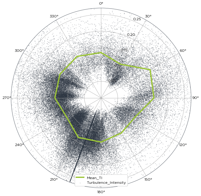
We can see a thick black line running along at 200 degrees. This would indicate that the wind vane was stuck for a long period of time and was not cleaned out. Using the cleaning methodology as outlined in Tutorial 5, we clean the data and then replot the data.

# specify location of existing cleaning file
Cleaning_Filepath = r'C:\Users\Stephen\Documents\Analysis\demo_cleaning_file.csv'
#Apply cleaning file to Raw Data
data = bw.apply_cleaning(data,Cleaning_Filepath)

Cleaning applied. (Please remember to assign the cleaned returned DataFrame to a variable.)

bw.TI.by_sector(data.Spd80mN,data.Spd80mNStd,data.Dir78mS)

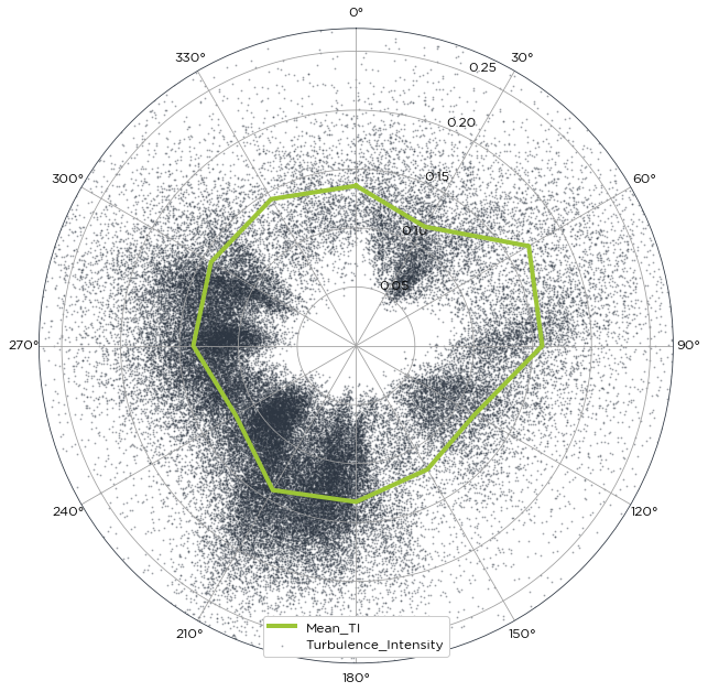
Wollah! the bad data has been cleaned out.

---

Calculate the turbulence intensity and plot by wind speed

Understanding the turbulence intensity by wind speed is an important metric when evaluating the site conditions of a potential wind farm site. The brightwind library has a function to compute this and plot against the IEC Turbulence classes and the mean and representative turbulence intensity. The mean speed and the standard deviation of the same mean speed are passed into the following function.

bw.TI.by_speed(data.Spd80mN,data.Spd80mNStd)

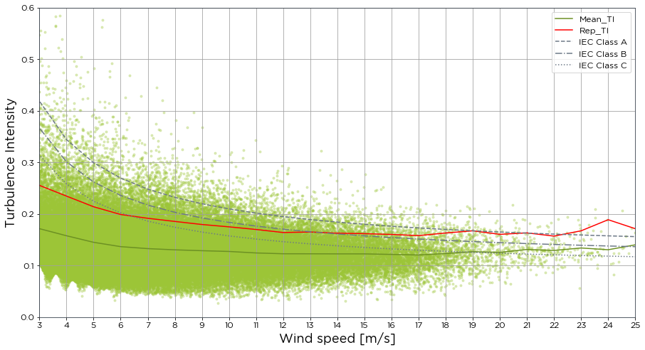
Returning the exact data from the plot can be useful especially when looking to extract inputs for turbulence intensity in Windfarmer or Openwind. To do this, we simply need to assign a plot and table to the function, and activiate the return_data flag within the function.

TI_plot, TI_Table = bw.TI.by_speed(data.Spd80mN, data.Spd80mNStd, return_data=True)
TI_Table

	Mean_TI	TI_Count	Rep_TI	TI_2Sigma	Char_TI
Speed Bin
3	0.171291	3429	0.255260	0.066981	0.193619
4	0.157540	7963	0.234453	0.061226	0.172846
5	0.144822	8852	0.213788	0.054829	0.155787
6	0.136418	9519	0.198752	0.049315	0.144637
7	0.132567	9594	0.191380	0.045464	0.139062
8	0.130207	8915	0.185284	0.043492	0.135643
9	0.128533	7631	0.179356	0.040206	0.133000
10	0.127061	6383	0.174785	0.037214	0.130782
11	0.124160	5240	0.169697	0.035074	0.127349
12	0.122585	4248	0.163811	0.033470	0.125374
13	0.122528	3315	0.164814	0.032269	0.125011
14	0.122377	2582	0.162472	0.030658	0.124566
15	0.122358	1933	0.161577	0.030678	0.124403
16	0.121319	1366	0.160051	0.029988	0.123193
17	0.120240	904	0.157809	0.028919	0.121941
18	0.123028	536	0.162825	0.029853	0.124687
19	0.126564	290	0.167137	0.030823	0.128187
20	0.125273	173	0.160253	0.026733	0.126610
21	0.130887	106	0.163101	0.023450	0.132004
22	0.129061	81	0.156819	0.022860	0.130100
23	0.133793	43	0.167104	0.025800	0.134915
24	0.130379	20	0.188619	0.033714	0.131784
25	0.139906	12	0.171210	0.033942	0.141264
26	0.114279	5	0.138046	0.025467	0.115259
27	0.133005	4	0.141158	0.010494	0.133394

---

Getting the 12x24 matrix of turbulence

The 12x24 matrix of turbulence is useful for seeing how the TI varies throughout the year. It shows the average turbulence for each hour of the day and for each month of the year.

bw.TI.twelve_by_24(data.Spd80mN, data.Spd80mNStd)

Month	1	2	3	4	5	6	7	8	9	10	11	12
Hour
0	0.123298	0.127858	0.132076	0.139142	0.139856	0.118668	0.142162	0.134350	0.127003	0.130014	0.120780	0.123587
1	0.123201	0.130815	0.136646	0.136444	0.149340	0.122524	0.130824	0.130241	0.131105	0.128241	0.116534	0.129366
2	0.127529	0.129643	0.136712	0.133500	0.139576	0.125087	0.128889	0.119857	0.123331	0.131344	0.119824	0.128259
3	0.126838	0.130400	0.136464	0.138197	0.141988	0.126567	0.127587	0.131554	0.126498	0.129808	0.127028	0.124243
4	0.135728	0.144298	0.144407	0.134473	0.141474	0.124459	0.125384	0.132680	0.126264	0.130177	0.117818	0.128227
5	0.130230	0.135277	0.139639	0.128773	0.128980	0.119023	0.127826	0.136850	0.120663	0.128160	0.115044	0.131810
6	0.126320	0.141140	0.141834	0.129834	0.135211	0.127730	0.135631	0.130856	0.128388	0.134495	0.119158	0.132965
7	0.131307	0.142126	0.137936	0.138492	0.137093	0.130571	0.140000	0.135732	0.132314	0.121811	0.126774	0.136691
8	0.124468	0.142668	0.141129	0.141683	0.149440	0.136717	0.143967	0.145758	0.136104	0.124737	0.123307	0.127271
9	0.126294	0.145591	0.143226	0.145519	0.150014	0.136577	0.143980	0.151626	0.142062	0.126898	0.121963	0.131016
10	0.130001	0.138173	0.141617	0.149271	0.161478	0.139885	0.144885	0.143630	0.147945	0.133367	0.127976	0.133389
11	0.132958	0.146347	0.145441	0.157493	0.155721	0.146634	0.144312	0.146676	0.154125	0.135837	0.128731	0.134031
12	0.132495	0.138591	0.145740	0.154551	0.158121	0.144148	0.145068	0.147703	0.151267	0.139552	0.139960	0.135619
13	0.135304	0.134754	0.145116	0.153083	0.153779	0.146184	0.147626	0.143644	0.146434	0.136658	0.130497	0.139250
14	0.130852	0.138478	0.146039	0.152753	0.156182	0.148084	0.144676	0.141140	0.143679	0.140105	0.131583	0.132048
15	0.126984	0.136637	0.148085	0.150065	0.155449	0.151128	0.139470	0.139497	0.148388	0.133079	0.141219	0.127299
16	0.129137	0.136645	0.144660	0.144193	0.152020	0.144948	0.143914	0.137312	0.149131	0.132714	0.135752	0.127104
17	0.131636	0.131892	0.137444	0.138432	0.146620	0.136568	0.136615	0.135192	0.138748	0.133199	0.133116	0.131362
18	0.125875	0.126344	0.125465	0.139556	0.140156	0.130648	0.133082	0.136368	0.134938	0.131969	0.124545	0.128202
19	0.121544	0.126259	0.127431	0.130534	0.135474	0.127702	0.133445	0.133482	0.127215	0.134546	0.120931	0.132309
20	0.128158	0.123049	0.131153	0.131193	0.131277	0.123628	0.132033	0.122578	0.128675	0.135552	0.124711	0.140587
21	0.127949	0.123772	0.126673	0.139372	0.129974	0.116301	0.122953	0.118066	0.124986	0.137319	0.130091	0.131600
22	0.131022	0.129903	0.131806	0.134071	0.129140	0.126089	0.127458	0.116963	0.128107	0.130918	0.128626	0.143479
23	0.122156	0.128121	0.126622	0.137240	0.141210	0.118557	0.136640	0.130691	0.133659	0.129783	0.124497	0.137975

---