How to apply a cleaning file¶

[1]:

# This cell is just used to record the date of this tutorial and is not part of the tutorial.
import datetime
print('Last updated: {}'.format(datetime.date.today().strftime('%d %B, %Y')))

Last updated: 19 July, 2019

Outline:¶

This guide will demonstrate how to use the apply_cleaning() and apply_cleaning_windographer() functions to clean data using pre-existing file which denote the cleaning to be applied. The tutorial includes the following steps:

1. ``apply_cleaning()`` with a simple csv:

import the brightwind library and some sample data
plot monthly means of raw wind speed
apply cleaning to data based on a pre-existing .csv cleaning file:
plot monthly means of cleaned wind speed
overview of cleaning file structure

2. ``apply_cleaning_windographer()`` with a windographer file:

import some sample data
plot monthly means of raw wind speed
apply cleaning to data based on a pre-existing windographer cleaning file:
plot monthly means of cleaned wind speed

1. `apply_cleaning()` with a simple csv:¶

Import the brightwind library and some sample data:¶

[2]:

import brightwind as bw

[3]:

# specify location of existing sample dataset
data_file_path = r'C:\Users\Stephen\Documents\Analysis\demo_data.csv'
# load data as dataframe
data = bw.load_csv(data_file_path)

# show first few rows of dataframe
data.head(5)

[3]:

	Spd80mN	Spd80mS	Spd60mN	Spd60mS	Spd40mN	Spd40mS	Spd80mNStd	Spd80mSStd	Spd60mNStd	Spd60mSStd	...	Dir78mSStd	Dir58mS	Dir58mSStd	Dir38mS	Dir38mSStd	T2m	RH2m	P2m	PrcpTot	BattMin
Timestamp
2016-01-09 15:30:00	8.370	7.911	8.160	7.849	7.857	7.626	1.240	1.075	1.060	0.947	...	6.100	110.1	6.009	112.2	5.724	0.711	100.0	935.0	0.0	12.94
2016-01-09 15:40:00	8.250	7.961	8.100	7.884	7.952	7.840	0.897	0.875	0.900	0.855	...	5.114	110.9	4.702	109.8	5.628	0.630	100.0	935.0	0.0	12.95
2016-01-09 17:00:00	7.652	7.545	7.671	7.551	7.531	7.457	0.756	0.703	0.797	0.749	...	4.172	113.1	3.447	111.8	4.016	1.126	100.0	934.0	0.0	12.75
2016-01-09 17:10:00	7.382	7.325	6.818	6.689	6.252	6.174	0.844	0.810	0.897	0.875	...	4.680	118.8	5.107	115.6	5.189	0.954	100.0	934.0	0.0	12.71
2016-01-09 17:20:00	7.977	7.791	8.110	7.915	8.140	7.974	0.556	0.528	0.562	0.524	...	3.123	115.9	2.960	113.6	3.540	0.863	100.0	934.0	0.0	12.69

5 rows × 29 columns

Plot monthly means of raw data:¶

[4]:

# create list of columns which include anemometer wind speed data
anemometers = ['Spd80mN', 'Spd80mS', 'Spd60mN', 'Spd60mS', 'Spd40mN', 'Spd40mS']

[5]:

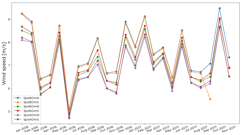
# plot monthly means of wind speed for each anemometer
bw.monthly_means(data[anemometers])

[5]:

../_images/tutorials_how_to_apply_a_cleaning_file_9_0.png

Note the spurious ‘Spd80mS’ monthly mean values which can be seen for the last few months.

Apply cleaning to data based on a pre-existing cleaning file:¶

[6]:

# specify location of associated cleaning file
cleaning_file_path = r'C:\Users\Stephen\Documents\Analysis\demo_cleaning_file.csv'

Data can be cleaned either in place or by assigning the cleaned data to a new variable. By deafult, the original data is untouched and a new DataFrame containing the cleaned data is created.

[7]:

# apply cleaning
clean_data = bw.apply_cleaning(data, cleaning_file_path)

To apply cleaning in place, i.e. replace the original data with the cleaned data, set the inplace parameter to True:

[8]:

# apply cleaning in place
bw.apply_cleaning(data, cleaning_file_path, inplace=True)

[8]:

	Spd80mN	Spd80mS	Spd60mN	Spd60mS	Spd40mN	Spd40mS	Spd80mNStd	Spd80mSStd	Spd60mNStd	Spd60mSStd	...	Dir78mSStd	Dir58mS	Dir58mSStd	Dir38mS	Dir38mSStd	T2m	RH2m	P2m	PrcpTot	BattMin
Timestamp
2016-01-09 15:30:00	NaN	NaN	NaN	NaN	NaN	NaN	NaN	NaN	NaN	NaN	...	NaN	NaN	NaN	NaN	NaN	NaN	NaN	NaN	NaN	NaN
2016-01-09 15:40:00	NaN	NaN	NaN	NaN	NaN	NaN	NaN	NaN	NaN	NaN	...	NaN	NaN	NaN	NaN	NaN	NaN	NaN	NaN	NaN	NaN
2016-01-09 17:00:00	NaN	NaN	NaN	NaN	NaN	NaN	NaN	NaN	NaN	NaN	...	NaN	NaN	NaN	NaN	NaN	NaN	NaN	NaN	NaN	NaN
2016-01-09 17:10:00	7.382	7.325	6.818	6.689	6.252	6.174	0.844	0.810	0.897	0.875	...	4.680	118.80	5.107	115.60	5.189	0.954	100.0	934.0	0.0	12.71
2016-01-09 17:20:00	7.977	7.791	8.110	7.915	8.140	7.974	0.556	0.528	0.562	0.524	...	3.123	115.90	2.960	113.60	3.540	0.863	100.0	934.0	0.0	12.69
2016-01-09 17:30:00	8.340	8.160	8.370	8.170	8.330	8.180	0.676	0.607	0.756	0.708	...	3.260	117.20	3.600	117.40	4.526	0.731	100.0	934.0	0.0	12.67
2016-01-09 17:40:00	8.130	7.929	8.090	7.895	7.972	7.788	0.557	0.507	0.534	0.498	...	3.677	115.90	3.371	115.90	3.515	0.852	100.0	933.0	0.0	12.68
2016-01-09 17:50:00	7.480	7.283	7.706	7.486	7.649	7.481	0.588	0.526	0.590	0.529	...	3.500	119.90	3.265	118.90	3.322	0.771	100.0	933.0	0.0	12.67
2016-01-09 18:00:00	7.554	7.452	7.484	7.359	7.578	7.456	0.734	0.681	0.631	0.573	...	3.061	113.90	2.663	111.40	2.789	0.913	100.0	933.0	0.0	12.65
2016-01-09 18:10:00	8.220	8.070	8.080	7.888	7.791	7.639	0.743	0.724	0.800	0.757	...	3.427	115.10	4.055	113.80	4.834	0.832	100.0	933.0	0.0	12.62
2016-01-09 18:20:00	9.420	9.270	9.660	9.470	9.570	9.450	0.482	0.438	0.566	0.522	...	2.431	119.50	2.454	117.40	3.017	0.549	100.0	933.0	0.0	12.61
2016-01-09 18:30:00	9.910	9.810	9.610	9.480	8.940	8.840	0.568	0.513	0.698	0.648	...	3.272	114.90	3.271	113.20	4.454	0.529	100.0	933.0	0.0	12.60
2016-01-09 18:40:00	10.390	10.340	10.260	10.110	9.840	9.760	0.683	0.640	0.710	0.696	...	4.405	110.90	4.308	109.30	4.776	0.589	100.0	933.0	0.0	12.60
2016-01-09 18:50:00	10.360	10.320	10.320	10.230	9.830	9.820	0.840	0.780	0.857	0.841	...	3.509	108.30	3.642	106.00	4.478	0.448	100.0	932.0	0.0	12.61
2016-01-09 19:00:00	9.950	9.880	10.050	9.970	9.910	9.870	0.561	0.469	0.639	0.547	...	3.601	102.30	3.085	100.70	3.954	0.701	100.0	932.0	0.0	12.60
2016-01-09 19:10:00	9.620	9.600	9.590	9.550	9.240	9.260	0.767	0.666	0.847	0.732	...	4.701	100.80	4.184	99.90	4.012	0.691	100.0	932.0	0.0	12.59
2016-01-09 19:20:00	9.590	9.600	9.510	9.460	9.270	9.270	0.615	0.571	0.795	0.760	...	5.744	109.30	5.838	105.20	5.478	0.711	100.0	932.0	0.0	12.58
2016-01-09 19:30:00	10.520	10.520	10.520	10.440	10.510	10.490	0.608	0.571	0.501	0.477	...	2.017	122.00	2.219	118.60	2.905	0.823	100.0	932.0	0.0	12.58
2016-01-09 19:40:00	8.970	8.950	9.190	9.100	9.260	9.190	0.691	0.617	0.705	0.659	...	3.884	123.10	4.036	119.20	3.911	0.913	100.0	931.0	0.0	12.57
2016-01-09 19:50:00	7.334	7.339	7.212	7.151	6.995	6.964	1.286	1.283	1.470	1.423	...	13.060	113.80	12.850	112.80	9.380	1.156	100.0	931.0	0.0	12.57
2016-01-09 20:00:00	5.310	5.445	4.788	4.901	4.093	4.190	1.202	1.190	1.259	1.226	...	16.890	92.30	16.320	82.10	20.130	1.317	100.0	931.0	0.0	12.56
2016-01-09 20:10:00	4.052	4.044	3.956	3.921	3.572	3.500	0.881	0.868	0.802	0.787	...	16.450	106.00	18.110	98.80	18.040	1.389	100.0	931.0	0.0	12.56
2016-01-09 20:20:00	3.632	3.519	3.653	3.584	3.594	3.524	0.816	0.787	0.658	0.615	...	11.660	95.00	10.780	90.90	10.660	1.288	100.0	931.0	0.0	12.55
2016-01-09 20:30:00	6.868	6.797	6.667	6.566	6.363	6.277	1.297	1.313	1.383	1.371	...	7.568	112.40	5.917	111.90	6.342	1.449	100.0	931.0	0.0	12.54
2016-01-09 20:40:00	3.496	3.462	4.098	4.110	4.252	4.318	1.363	1.367	1.616	1.593	...	13.770	104.30	12.860	106.20	12.810	1.317	100.0	931.0	0.0	12.54
2016-01-09 20:50:00	2.390	2.394	2.033	2.000	1.402	1.347	0.774	0.706	0.725	0.682	...	21.640	98.70	33.320	78.95	39.480	0.913	100.0	931.0	0.0	12.54
2016-01-09 21:00:00	3.002	3.042	2.509	2.521	2.252	2.156	1.313	1.265	1.237	1.285	...	22.610	73.82	25.350	56.03	33.450	1.338	100.0	931.0	0.0	12.53
2016-01-09 21:10:00	3.489	3.448	3.061	3.031	2.874	2.851	0.821	0.793	0.632	0.575	...	10.750	74.83	11.530	66.91	12.570	1.176	100.0	930.0	0.0	12.53
2016-01-09 21:20:00	4.204	4.321	3.661	3.715	2.972	3.074	0.995	0.924	1.049	1.005	...	10.920	83.60	11.370	75.78	14.990	1.236	100.0	930.0	0.0	12.52
2016-01-09 21:30:00	6.486	6.648	5.745	5.879	4.862	5.021	1.224	1.237	1.329	1.329	...	12.640	69.43	12.760	65.76	14.290	1.398	100.0	930.0	0.0	12.52
...	...	...	...	...	...	...	...	...	...	...	...	...	...	...	...	...	...	...	...	...	...
2017-11-23 06:00:00	10.620	NaN	10.420	10.370	10.110	10.030	0.857	NaN	0.803	0.752	...	NaN	NaN	NaN	257.20	4.303	0.589	100.0	940.0	0.1	12.71
2017-11-23 06:10:00	10.720	NaN	10.670	10.600	10.470	10.380	1.027	NaN	0.938	0.919	...	NaN	NaN	NaN	258.70	4.351	0.701	100.0	940.0	0.0	12.71
2017-11-23 06:20:00	10.940	NaN	10.650	10.600	10.290	10.210	0.708	NaN	0.823	0.778	...	NaN	NaN	NaN	257.70	3.923	0.761	99.5	940.0	0.0	12.71
2017-11-23 06:30:00	10.270	NaN	10.130	9.960	9.910	9.790	0.800	NaN	0.865	0.808	...	NaN	NaN	NaN	251.60	3.722	0.792	98.0	940.0	0.0	12.71
2017-11-23 06:40:00	8.180	NaN	7.985	7.811	7.649	7.519	1.167	NaN	1.239	1.199	...	NaN	NaN	NaN	242.80	4.858	0.518	98.2	941.0	0.0	12.71
2017-11-23 06:50:00	8.870	NaN	8.570	8.330	8.020	7.873	0.676	NaN	0.582	0.534	...	NaN	NaN	NaN	232.90	3.426	0.782	99.9	941.0	0.0	12.71
2017-11-23 07:00:00	9.300	NaN	8.950	8.670	8.590	8.400	0.933	NaN	0.994	0.937	...	NaN	NaN	NaN	229.30	4.575	0.761	99.5	941.0	0.0	12.71
2017-11-23 07:10:00	8.130	NaN	7.863	7.592	7.283	7.094	0.823	NaN	0.837	0.794	...	NaN	NaN	NaN	225.10	4.478	0.721	99.9	941.0	0.0	12.67
2017-11-23 07:20:00	8.910	NaN	8.500	8.250	8.020	7.864	1.063	NaN	0.977	0.929	...	NaN	NaN	NaN	226.70	5.236	0.751	100.0	941.0	0.0	12.66
2017-11-23 07:30:00	9.610	NaN	9.260	8.980	8.630	8.470	0.942	NaN	0.923	0.860	...	NaN	NaN	NaN	228.10	5.127	0.670	100.0	941.0	0.0	12.66
2017-11-23 07:40:00	10.900	NaN	10.310	10.050	9.680	9.490	1.268	NaN	1.170	1.111	...	NaN	NaN	NaN	232.70	5.563	0.570	100.0	941.0	0.0	12.67
2017-11-23 07:50:00	11.560	NaN	11.080	10.790	10.400	10.190	1.022	NaN	1.114	1.067	...	NaN	NaN	NaN	238.60	4.363	0.751	100.0	941.0	0.0	12.70
2017-11-23 08:00:00	11.730	NaN	11.290	11.030	10.690	10.490	0.842	NaN	0.834	0.759	...	NaN	NaN	NaN	237.40	3.395	0.771	100.0	941.0	0.0	12.70
2017-11-23 08:10:00	11.700	NaN	11.420	11.130	11.030	10.830	0.764	NaN	0.727	0.673	...	NaN	NaN	NaN	235.90	3.391	0.863	99.7	941.0	0.0	12.66
2017-11-23 08:20:00	12.270	NaN	12.020	11.760	11.510	11.330	0.774	NaN	0.800	0.755	...	NaN	NaN	NaN	237.00	3.657	0.842	99.5	941.0	0.0	12.66
2017-11-23 08:30:00	11.510	NaN	11.260	10.990	10.740	10.530	0.956	NaN	0.903	0.857	...	NaN	NaN	NaN	234.60	3.988	0.701	99.3	942.0	0.0	12.65
2017-11-23 08:40:00	11.380	NaN	10.850	10.520	10.310	10.090	0.962	NaN	0.867	0.840	...	NaN	NaN	NaN	235.00	4.448	0.751	99.7	942.0	0.0	12.68
2017-11-23 08:50:00	10.420	NaN	10.090	9.810	9.590	9.380	1.034	NaN	1.141	1.111	...	NaN	NaN	NaN	223.70	7.394	0.680	99.7	942.0	0.0	12.69
2017-11-23 09:00:00	9.050	NaN	8.530	8.270	7.696	7.503	0.668	NaN	0.763	0.681	...	NaN	NaN	NaN	211.60	7.172	0.812	100.0	942.0	0.0	12.70
2017-11-23 09:10:00	7.484	NaN	7.231	6.956	6.596	6.404	1.009	NaN	0.868	0.811	...	NaN	NaN	NaN	213.00	7.851	0.771	98.4	942.0	0.0	12.69
2017-11-23 09:20:00	7.228	NaN	6.903	6.691	6.273	6.089	0.756	NaN	0.841	0.753	...	NaN	NaN	NaN	209.10	7.654	0.549	99.0	943.0	0.0	12.70
2017-11-23 09:30:00	7.740	NaN	7.359	7.147	6.889	6.775	0.634	NaN	0.618	0.586	...	NaN	NaN	NaN	221.00	6.078	0.711	99.6	943.0	0.0	12.52
2017-11-23 09:40:00	8.380	NaN	7.900	7.675	7.190	7.068	0.822	NaN	0.881	0.798	...	NaN	NaN	NaN	221.90	4.969	0.651	98.8	943.0	0.0	12.73
2017-11-23 09:50:00	9.870	NaN	9.250	8.970	8.450	8.250	0.954	NaN	0.878	0.805	...	NaN	NaN	NaN	220.20	5.269	0.873	99.8	943.0	0.0	12.89
2017-11-23 10:00:00	9.800	NaN	9.340	9.070	8.630	8.450	1.170	NaN	1.136	1.076	...	NaN	NaN	NaN	221.90	5.125	0.731	98.6	943.0	0.0	12.94
2017-11-23 10:10:00	10.480	NaN	10.190	9.890	9.590	9.420	0.720	NaN	0.733	0.668	...	NaN	NaN	NaN	222.20	4.111	0.943	99.7	943.0	0.0	13.02
2017-11-23 10:20:00	9.390	NaN	9.120	8.850	8.520	8.340	0.659	NaN	0.734	0.651	...	NaN	NaN	NaN	218.40	4.817	0.792	98.6	943.0	0.0	13.69
2017-11-23 10:30:00	9.140	NaN	8.700	8.450	8.030	7.875	0.689	NaN	0.821	0.732	...	NaN	NaN	NaN	216.00	5.784	0.802	100.0	943.0	0.0	13.86
2017-11-23 10:40:00	7.927	NaN	7.383	7.159	6.811	6.668	0.817	NaN	0.769	0.692	...	NaN	NaN	NaN	219.50	5.051	0.883	100.0	943.0	0.0	13.80
2017-11-23 10:50:00	7.120	NaN	6.617	6.404	5.865	5.749	0.537	NaN	0.534	0.450	...	NaN	NaN	NaN	222.40	4.902	0.802	100.0	944.0	0.0	13.71

95629 rows × 29 columns

Plot monthly means of cleaned wind speed:¶

[9]:

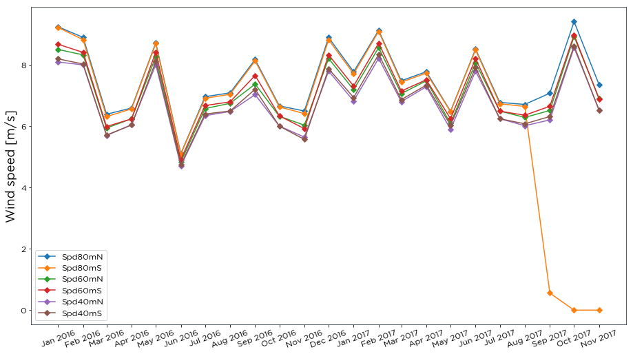
# plot monthly means of wind speed for each anemometer
bw.monthly_means(clean_data[anemometers])

[9]:

../_images/tutorials_how_to_apply_a_cleaning_file_18_0.png

Note that the spurious ‘Spd80mS’ values have been removed.

Overview of cleaning file structure:¶

[10]:

# load cleaning file
cleaning_file = bw.load_cleaning_file(cleaning_file_path)

# show cleaning file
cleaning_file

[10]:

	Sensor	Start	Stop	Reason
0	All	2016-01-09 15:30:00	2016-01-09 17:10:00	Installation
1	Spd	2016-03-09 06:20:00	2016-03-09 10:30:00	Icing
2	Dir	2016-03-09 06:20:00	2016-03-09 10:30:00	Icing
3	Spd	2016-03-29 23:50:00	2016-03-30 07:10:00	Icing
4	Dir	2016-03-29 23:50:00	2016-03-30 07:10:00	Icing
5	Spd	2016-11-08 02:30:00	2016-11-08 10:50:00	Icing
6	Dir	2016-11-08 02:30:00	2016-11-08 10:50:00	Icing
7	Spd	2016-11-18 15:50:00	2016-11-19 10:30:00	Icing
8	Dir	2016-11-18 15:50:00	2016-11-19 10:30:00	Icing
9	Spd	2016-11-20 16:40:00	2016-11-21 12:40:00	Icing
10	Dir	2016-11-20 16:40:00	2016-11-21 12:40:00	Icing
11	Spd	2017-01-21 00:00:00	2017-01-21 07:10:00	Icing
12	Dir	2017-01-21 00:00:00	2017-01-21 07:10:00	Icing
13	Spd	2017-01-28 14:10:00	2017-01-28 17:30:00	Icing
14	Dir	2017-01-28 14:10:00	2017-01-28 17:30:00	Icing
15	Spd	2017-10-30 01:40:00	2017-10-30 07:00:00	Icing
16	Dir	2017-10-30 01:40:00	2017-10-30 07:00:00	Icing
17	Dir58mS	2016-12-26 07:00:00	2018-02-09 21:30:00	Invalid
18	Dir78mS	2017-08-11 02:10:00	2018-02-09 21:30:00	Invalid
19	Spd80mS	2017-09-04 00:30:00	2018-02-09 21:30:00	Invalid

Each row of the cleaning file relates to a portion of the time series which has been flagged for quality reasons.
The ‘Sensor’ column specifies which variables are affected by the issue.
- The function looks for all column names in your data that contain the sensor name. Therefore, when the sensor name is just ‘Spd’ it will find ALL column names that contain ‘Spd’ and clean out the data.
- The sensor name ‘All’ is a special name which cleans ALL the data for that period.
The ‘Start’ and ‘Stop’ dates specify the length the time period to be removed. The flagged data is inclusive of the ‘start’ time, and ends before the ‘stop’ time.
The ‘Reason’ field justifies why the data should be removed.

2. `apply_cleaning_windographer()` with a windographer file:¶

Import some sample data:¶

[11]:

# specify location of existing sample dataset
campbell_data_file_path = r'C:\Users\Stephen\Documents\Analysis\campbell_scientific_demo_data.csv'

# load data as dataframe
campbell_data = bw.load_campbell_scientific(campbell_data_file_path)

# show first few rows of dataframe
campbell_data.head(5)

[11]:

	RECORD	Site	LoggerID	Spd80mN	Spd80mS	Spd60mN	Spd60mS	Spd40mN	Spd40mS	Spd80mNStd	...	Dir78mSStd	Dir58mS	Dir58mSStd	Dir38mS	Dir38mSStd	T2m	RH2m	P2m	PrcpTot	BattMin
Timestamp
2016-01-09 15:30:00	0	demo_mast	7000	8.370	7.911	8.160	7.849	7.857	7.626	1.240	...	6.100	110.1	6.009	112.2	5.724	0.711	100.0	935.0	0.0	12.94
2016-01-09 15:40:00	1	demo_mast	7000	8.250	7.961	8.100	7.884	7.952	7.840	0.897	...	5.114	110.9	4.702	109.8	5.628	0.630	100.0	935.0	0.0	12.95
2016-01-09 17:00:00	2	demo_mast	7000	7.652	7.545	7.671	7.551	7.531	7.457	0.756	...	4.172	113.1	3.447	111.8	4.016	1.126	100.0	934.0	0.0	12.75
2016-01-09 17:10:00	3	demo_mast	7000	7.382	7.325	6.818	6.689	6.252	6.174	0.844	...	4.680	118.8	5.107	115.6	5.189	0.954	100.0	934.0	0.0	12.71
2016-01-09 17:20:00	4	demo_mast	7000	7.977	7.791	8.110	7.915	8.140	7.974	0.556	...	3.123	115.9	2.960	113.6	3.540	0.863	100.0	934.0	0.0	12.69

5 rows × 32 columns

Plot monthly means of raw wind speed:¶

[12]:

# plot monthly means of wind speed for each anemometer
bw.monthly_means(campbell_data[anemometers])

[12]:

../_images/tutorials_how_to_apply_a_cleaning_file_27_0.png

You can see here that the data is the same as example 1, just loaded in a different format.

Apply cleaning to data based on a pre-existing windographer cleaning file:¶

Cleaning can also be applied to windographer files, by passing inplace=True to the apply_cleaning_windographer function. By default, inplace=False and the cleaned data must be assigned to a new variables, as below:

[13]:

# specify location of associated cleaning file
windog_log_file_path = r'C:\Users\Stephen\Documents\Analysis\windographer_flagging_log.txt'

# apply cleaning
campbell_data_clean = bw.apply_cleaning_windographer(campbell_data, windog_log_file_path)

Plot monthly means of cleaned wind speed:¶

[14]:

# plot monthly means of wind speed for each anemometer
bw.monthly_means(campbell_data_clean[anemometers])

[14]:

../_images/tutorials_how_to_apply_a_cleaning_file_33_0.png

As with example 1, the spurious data has been removed.

How to apply a cleaning file¶

Outline:¶

1. apply_cleaning() with a simple csv:¶

Import the brightwind library and some sample data:¶

Plot monthly means of raw data:¶

Apply cleaning to data based on a pre-existing cleaning file:¶

Plot monthly means of cleaned wind speed:¶

Overview of cleaning file structure:¶

2. apply_cleaning_windographer() with a windographer file:¶

Import some sample data:¶

Plot monthly means of raw wind speed:¶

Apply cleaning to data based on a pre-existing windographer cleaning file:¶

Plot monthly means of cleaned wind speed:¶

1. `apply_cleaning()` with a simple csv:¶

2. `apply_cleaning_windographer()` with a windographer file:¶